Why MLX is Important for the ML Community

And a step-by-step guide to train a machine learning model on your Mac

May 07, 2024

MLX is a lot bigger deal for the machine learning community than most people think. Let’s understand what it is and what it means, and let’s even get it up-and-running on your Mac.

What is MLX?

MLX is a machine learning framework built specifically for Apple Silicon. This gives researchers (including individuals and hobbyists) the ability to train and run machine learning models on their Mac. MLX uses syntax similar to NumPy to make it feel intuitive for anyone already performing computation with Python.

Important links:

It’s important to note: MLX is focused on machine learning research, not production-level deployment.

Why is MLX important?

MLX greatly increases the accessibility of machine learning. I know I mention ML accessibility a lot, but isn’t mentioned enough. Accessibility is important from a consumer standpoint so we can get more people using ML in their daily lives, but it’s also important from a research and development standpoint. More ML researchers and engineers is good for everyone.

Up until recently, running ML models locally required a windows PC with a Nvidia graphics card for a proper out-of-the-box solution. I know many researchers who have both a Mac for generally purpose development and a PC specifically for their ML workflows. The necessity of a PC and purpose-built graphics card has created a huge barrier of entry to machine learning, especially for researchers in developing countries. This barrier of entry increases as the demand for Nvidia GPUs increases (think about how hard it was to get one during the crypto boom). Making ML accessible on more hardware (especially hardware many interested in machine learning may already have) is a huge win.

Sure, a PC and Nvidia card is still more powerful for machine learning than using MLX, but it isn’t a necessity to run heavy-duty models locally—large models will run on cloud-based solutions. Local models are more useful for spinning up quick tests using smaller models, which MLX and Apple silicon handle perfectly.

Let’s use MLX

Let’s set up a really simple neural network using MLX and Python. My go-to basic example is training a MNIST perceptron. It teaches a small machine learning model to recognize handwritten digits. This was the first ML model I ever trained and it made me super excited about machine learning because it’s simple but showcases the utility of machine learning.

As I was writing this section, I was putting together my own data loader for training on MNIST and I realized that MLX uses MNIST as one of their examples in their documentation. Instead of working from scratch, we’ll walk through their guide but I’ll split it into the general steps for setting up a model for training. The full MLX guide is here.

1. Setup and Prerequisites

While you don’t need any prior knowledge to follow this tutorial if you want to copy and paste, here are a few prerequisites you’ll find helpful:

You need a Mac with Apple silicon (this is a MUST - an Intel Mac won’t work).
A basic understanding of neural networks and machine learning.
Some familiarity with Python.

If you find there are basic concepts throughout this guide you don’t understand, you can check out my machine learning road map to learn them. It takes you through machine learning prerequisites and machine learning math for free.

To start setting up, you’ll need a Python version >=3.8 and a MacOS version >= 13.5. Install MLX via pip:

pip install mlx

Install NumPy via pip, too:

pip install numpy

2. Data Preparation

The first step of creating a machine learning model is having the right data. This requires understanding the data you need for training, acquiring it, and properly loading it into your model.

For this example, we’re going to use the MNIST dataset. This a predefined dataset of 70,000 images of handwritten numbers that have been normalized and centered. The dataset also includes labels detailing which number each image represents.

There are many datasets like MNIST that have been put together by the machine learning community to make training models easier. Data collection is the most difficult problem within machine learning. ML models require a lot of data to achieve a remarkable level of performance. This data needs to be clear, meaningful, and often labeled. “Preprocessing” data is a tedious task often done by hand. This manual process includes organizing, normalizing, labeling, and transforming the data into the inputs a ML model requires. Datasets put together by the machine learning community make this much easier.

Let’s grab our MNIST dataset. Usually, this requires downloading training and test files from the internet (I’ve grabbed MNIST from Kaggle before) then creating a data loader class that pulls those files into the program, modifies them as needed, and loads them into the model. Luckily, we don’t have to do any of that. The MLX team has already written a data loader for MNIST that retrieves the MNIST files for us.

Create a Python file called mnist.py and copy the MLX team’s data loader into that file.

3. Model Definition

Create a main.py file to set up our model and run our training loop. This next section will primarily be pulled from the MLX documentation with a few things moved around. If you want to compare your code as you put it together to functional example code you can check out my code or the MLX team’s code.

First we’ll start with our Python imports to use MLX and NumPy:

import mlx.core as mx
import mlx.nn as nn
import mlx.optimizers as optim
import numpy as np
import argparse

Next, we’ll create the model as its own class, using an __init__ where parameters and submodules are set up and a __call__ where the computation for the model is implemented:

class MLP(nn.Module):

    def __init__(
        self, num_layers: int, input_dim: int, hidden_dim: int, output_dim: int):
        super().__init__()

        layer_sizes = [input_dim] + [hidden_dim] * num_layers + [output_dim]
        self.layers = [
            nn.Linear(idim, odim)
            for idim, odim in zip(layer_sizes[:-1], layer_sizes[1:])
        ]

    def __call__(self, x):
        for l in self.layers[:-1]:
            x = mx.maximum(l(x), 0.0)
        return self.layers[-1](x)

Next, we’ll set up our model parameters and load our data. This requires creating a main function and adding this code to the start of that function:

num_layers = 2
hidden_dim = 32
num_classes = 10
batch_size = 256
num_epochs = 10
learning_rate = 1e-1

# Load the data
import mnist
train_images, train_labels, test_images, test_labels = map(
    mx.array, mnist.mnist()
)

At this point, we’re ready to set up training.

4. Training

Now that our model is defined, let’s define our loss and accuracy functions (outside of the main function):

def loss_fn(model, X, y):
  return mx.mean(nn.losses.cross_entropy(model(X), y))

def eval_fn(model, X, y):
  return mx.mean(mx.argmax(model(X), axis=1) == y)

Set up our optimizer and create an iterator that separates our data into the appropriate batches for training (this should also be outside of the main function):

def batch_iterate(batch_size, X, y):
    perm = mx.array(np.random.permutation(y.size))
    for s in range(0, y.size, batch_size):
        ids = perm[s : s + batch_size]
        yield X[ids], y[ids]

Finally, we define our training loop to put everything together:

# Load the model
model = MLP(num_layers, train_images.shape[-1], hidden_dim, num_classes)
mx.eval(model.parameters())

# Get a function which gives the loss and gradient of the
# loss with respect to the model's trainable parameters
loss_and_grad_fn = nn.value_and_grad(model, loss_fn)

# Instantiate the optimizer
optimizer = optim.SGD(learning_rate=learning_rate)

for e in range(num_epochs):
    for X, y in batch_iterate(batch_size, train_images, train_labels):
        loss, grads = loss_and_grad_fn(model, X, y)

        # Update the optimizer state and model parameters
        # in a single call
        optimizer.update(model, grads)

        # Force a graph evaluation
        mx.eval(model.parameters(), optimizer.state)

    accuracy = eval_fn(model, test_images, test_labels)
    print(f"Epoch {e}: Test accuracy {accuracy.item():.3f}")

5. Evaluation

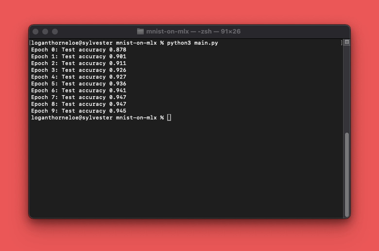
Now we can train our model! While we train the model, we’ll periodically evaluate its performance. In our example, we do this at the end of each epoch. Running main.py:

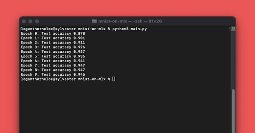
python3 main.py

should generate output that looks like this:

And that’s your first model trained using MLX! You’ll notice the accuracy of the model goes up over each iteration of the training data. This is what we want to see. If this isn’t increasing, then something is going wrong. If you have questions about setting this up, leave a comment on this article or reach out to me on X or LinkedIn.

That’s all for today. I’ve already got some great ML resources to share this Friday. If you’re interested in supporting Society’s Backend, you can do so for just $1/mo for your first year:

Get 80% off for 1 year

Thanks for reading!